
| Approved by: | ______________________________________________________ |
| Dr. Charles K. Shank, Assistant Professor | |
| ______________________________________________________ | |
| Dr. Tony H. Chang, Professor | |
| ______________________________________________________ | |
| Dr. Roy S. Czernikowski, Professor and Department Head | |
Title: A Petri Net Design, Simulation, and Verification Tool
I, Richard Scott Brink, hereby grant permission to the Wallace
Memorial Library to reproduce my thesis in whole or part.
Signature: __________________________
Date: ______________________________
| Aptiva | Aptiva is a trademark of International Business Machines |
| HP | HP is a trademark of the Hewlett-Packard Company |
| IBM | IBM is a trademark of International Business Machines |
| Java | Java is a trademark of Sun Microsystems, Inc. |
| Macintosh | Macintosh is a trademark of Apple Computer, Inc. |
| Solaris | Solaris is a trademark of Sun Microsystems, Inc. |
| Symantec Café | Symantec Café is a trademark of Symantec Corporation |
| Windows 95 | Windows 95 is a trademark of Microsoft Corporation |
I would like to thank my parents, Lee and Suzie Brink for their
support throughout my college career and making this culmination
of my educational experience possible. This thesis is dedicated
to them.
Increasing desire for thorough simulation and analysis of engineered
products is quickly replacing the prototype and test design model.
Petri nets are important instruments for modeling concurrent,
distributed, asynchronous, parallel, deterministic, and non-deterministic
systems. This tool provides designers with the ability to easily
specify a Petri net design with an easy to use user interface,
then simulate and analyze the Petri net to determine essential
design properties using the reachability tree technique. The tool
will construct a reachability tree, then analyze the tree for
properties of safeness, boundedness, liveness, and conservativeness.
| Arc | An arc is a Petri net component which relates places to transitions and transitions to places, thus forming an input function and an output function for each transition. Arcs are generally represented as a directed line in a Petri net design. An arc also has an associated weight, representing the number of tokens needed to enable the arc. |
| AWT | Abstract Windowing Toolkit. A platform independent interface for creating window components for user interfaces such as windows, buttons, menus, scrollbars, etc. |
| Bounded | A place is k-bounded when, for each marking in a reachability tree, the maximum number of tokens appearing in that place never exceeds k. A Petri net is j-bounded if all places in the net are bounded and j represents the maximum bound value of all places in the net. |
| Café | An Integrated Development and Debugging Environment (IDDE) created by the Symantec Corporation for the development of Java programs. |
| Duplicate Node | A duplicate node is a marking that is already present in a reachability tree and need not be analyzed during the construction of the reachability tree because all successors to the node will have already been generated from the first occurrence of the marking. |
| Conservative | A Petri net is said to be strictly conservative if, for all possible markings, the total number of tokens in the Petri net always remains constant. A Petri net may also be conservative with respect to a weighting vector such that all markings when multiplied by the weighting vector are equal. |
| Frontier Node | A frontier node is a marking generated during the construction of a reachability tree that has not yet been analyzed to find its successors. |
| GUI | Graphical User Interface |
| HTML | HyperText Markup Language |
| IDDE | Integrated Development and Debugging Environment |
| Initial Marking | An Initial Marking is an assignment of a tokens to places that defines the starting state of the Petri net. |
| Input Function | An input function I is a mapping of transition tj to a collection of places I(tj), known as the input places of the transition. (Peterson, 1981). |
| Java | Java is an interpreted, object oriented, portable, multithreaded programming language with a C/C++ look and feel. |
| JDK | Java Development Kit. A set of tools by Sun Microsystems including compiler, interpreter, documentation generator, etc. for the development of Java programs. |
| JVM | Java Virtual Machine. A virtual machine for processing Java bytecodes. |
| Layout Manager | A tool for creating hardware independent arrangements of graphical components in a Java program. |
| Live | A Petri net is live when there exist no terminal nodes in the net's reachability tree. For each marking in the reachability tree, there exists at least one transition that is enabled for that marking. |
| Marking | A mapping of tokens to places which defines a state for the Petri net. |
| Ordinary Petri Net | An ordinary Petri net contains only arcs with a weight of one. |
| Output Function | An output function O is a mapping of transition tj to a collection of places O(tj), known as the output places of the transition. (Peterson, 1981). |
| Petri Net | A Petri net is a graphical and mathematical modeling tool which is able to model concurrent, asynchronous, distributed, and parallel systems. The basic Petri net consists of four different components: Places, Transitions, Arcs, and Tokens. |
| Place | A Place is a basic Petri net component which represents a condition. If a place is a member of the input function of a transition, it is a pre-condition for that transition, or event, to occur. If a place is a member of the output function of a transition, it is a post-condition of the event or transition firing. A place is generally represented by a circle in a Petri net design. |
| Reachability Tree | A reachability tree represents all of the obtainable markings for a Petri net. The tree begins with the initial marking, with a line from the initial marking to a new marking for each enabled transition. The process is repeated for each new marking that is neither a terminal node or a duplicate node until all possible markings are found. |
| Safe | A place is said to be safe if, for all possible markings, the number of tokens in that place never exceeds one. The Petri net is declared safe if all of the places in the net are safe. |
| State-Space Explosion | The effect where the number of possible states in a design increases exponentially as new elements are added to the design. |
| Terminal Node | A terminal node is a marking generated during the construction of a reachability tree that has no enabled transitions, and thus stops the growth of the tree through that node. |
| Token | A token is a basic Petri net component which is thought of as residing in a 'place'. A token signifies that a particular place, or condition, is true. Multiple tokens residing in a place are usually representative of the existence of multiple resources, rather than boolean conditions. |
| Transition | A transition is a basic Petri net component which represents an event. The event may occur when all of the input places to the transition contain enough tokens to enable the input arcs to the transition. The occurrence of the event, also known as a firing of the transition, will result in tokens being deposited through each of the output arcs of the transition into the respective output places. |
| Windows 95 | An operating system for IBM PCs and compatibles. |
In the engineering discipline, the complexity of systems are growing at a fast pace, with the industry becoming more and more cost competitive. Due to time and money constraints, it is no longer feasible to follow the design cycle of trial and error prototyping. Instead, the trend of designs today is leaning more toward simulation, and in some cases formal specification of a design, so that design flaws can be worked out before a prototype is even built. It is here that Petri nets are being used more and more frequently. However, what is needed for this approach to be effective is a good interface to design these Petri net models, with analysis and simulation functionality which will reduce design time and help the designer eliminate design flaws. It is this niche that the PetriTool application has been targeted for.
Petri nets have an origin dating back to 1962, when Carl Adam Petri wrote his PhD on the subject. Since that time, Petri nets have been accepted as a powerful formal specification tool for a variety of systems including concurrent, distributed, asynchronous, parallel, deterministic and non-deterministic. Petri nets also have applications in a number of different disciplines including engineering, manufacturing, business, chemistry, mathematics, and even within the judicial system.
Since their inception, there have been scores of variations on the initial structure of Petri nets, but most of these variations are simply additions to the basic definition of a Petri net. The basic Petri net structure consists of a finite set of places, a finite set of transitions, a finite set of arcs, and a set of tokens defining an Initial Marking. The set of arcs define two types of functions: input functions and output functions. These functions describe the flow of tokens from places to transitions and from transitions to places.
Figure 1 shows an example of a Petri net which models a producer-consumer problem that was designed using the PetriTool application. On the left is a producing entity, and on the right is the consumer entity. In the center is a buffer which allows up to sixteen items to be produced at a time. Once the producer produces sixteen items, the buffer is full and the producer will not be able to produce any more items until the consumer consumes at least one item.
This Petri net has a set of eight places, labeled P0 through P7. It also has a set of six transitions labeled T0 through T5. All of the arcs in this example are enabled by a single token. The Initial Marking for this Petri net is (1, 0, 0, 0, 16, 1, 0, 0) which is determined by noting the number of tokens in each place from P0 to P7 respectively. Notice that the number of tokens in each place is noted under the place with a text label "T=1" to represent one token or "T=16" to represent the presence of sixteen tokens. If the place contains no tokens, the label is omitted.
Once a Petri net has been drawn, it is important to be able to analyze the net to determine what sort of properties it has in order to determine if the design will be feasible for a particular application. The first step of analysis usually consists of forming a reachability tree. An example of a portion of the reachability tree for Figure 1 is shown in Figure 2.
| (1,0,0,0,16,1,0,0) | (0,1,0,0,16,1,0,0) | |
| (0,1,0,0,16,1,0,0) | (0,0,1,1,15,1,0,0) | |
| (0,0,1,1,15,1,0,0) | (1,0,0,1,15,1,0,0) | |
| (0,0,1,0,16,0,1,0) | ||
| (1,0,0,1,15,1,0,0) | (0,1,0,1,15,1,0,0) | |
| (1,0,0,0,16,0,1,0) | ||
| (0,0,1,0,16,0,1,0) | (1,0,0,0,16,0,1,0) | |
| (0,0,1,0,16,0,0,1) | ||
| (0,1,0,1,15,1,0,0) | (0,0,1,2,14,1,0,0) | |
| (0,1,0,0,16,0,1,0) | ||
| (1,0,0,0,16,0,1,0) | (0,1,0,0,16,0,1,0) | |
| (1,0,0,0,16,0,0,1) | ||
| (0,0,1,0,16,0,0,1) | (1,0,0,0,16,0,0,1) | |
| (0,0,1,0,16,1,0,0) | ||
| (0,0,1,2,14,1,0,0) | (1,0,0,2,14,1,0,0) | |
| (0,0,1,1,15,0,1,0) | ||
| (0,1,0,0,16,0,1,0) | (0,0,1,1,15,0,1,0) | |
| (0,1,0,0,16,0,0,1) | ||
| (1,0,0,0,16,0,0,1) | (0,1,0,0,16,0,0,1) | |
| (1,0,0,0,16,1,0,0)* | ||
| (0,0,1,0,16,1,0,0) | (1,0,0,0,16,1,0,0)* |
The reachability tree begins with the initial marking, in this case (1, 0, 0, 0, 16, 1, 0, 0). From this marking, a new marking is created for each enabled transition from that marking. In this case, there is only one enabled transition, T0, which results in a marking of (0, 1, 0, 0, 16, 1, 0, 0). Subsequently, a new marking is created for each enabled transition from the marking (0, 1, 0, 0, 16, 1, 0, 0), and the process repeats. Once a marking is found that is already present in the tree, it is marked (with an asterisk in the PetriTool application) and that marking need not be added to the tree a second time. This is known as a duplicate node. Once all possible markings have been found, the tree is complete. The completed reachability tree shows all of the possible markings that can be obtained from the initial marking given every possible sequence of transition firings.
Once the reachability tree is constructed, the tree can be analyzed in order to determine specific properties of the Petri net. Some of the more important properties that can be determined include safeness, boundedness, liveness, and conservativeness.
The property of safeness can be determined for both individual places and for the entire net. A place is said to be safe if, for all possible markings, the number of tokens in that place never exceeds one. The Petri net is declared safe if all of the places in the net are safe.
The property of boundedness can also be determined for individual places and for the entire Petri net. The boundedness property is actual a more general form of the safeness property. A place is said to be k-bounded if, for all possible markings, the number of tokens in that place never exceeds k. A Petri net is k-bounded if, for all possible markings, the number of tokens in any individual place in the net never exceeds k. Both the safe and bound properties for Petri nets are important in the field of engineering because they help determine what size buffers, counters, etc. are needed in order to implement the design. For instance, if all of the places are safe, it would be possible to implement these conditions with a boolean variable. If a place is representative of a buffer, and is 16-bounded, then the designer knows to use a buffer of size 16.
The third property, liveness, is one of the most important properties of the Petri net for most applications. The liveness property encapsulates the concept of a system which will be able to run continuously, i.e. a system which does not deadlock, which is an important property when modeling operating systems, communication protocols, computer programs, and just about any safety critical system. Using the most general definition of liveness, a Petri net is considered live if, for all possible markings, there is always a transition enabled. There have been, however, many other concepts developed in the area of liveness, some of which define different levels of liveness for individual transitions (Murata, 1989).
The last property, conservativeness, is associated with the total number of tokens within the Petri net. A Petri net is said to be strictly conservative if, for all possible markings, the total number of tokens in the Petri net always remains constant. A Petri net can also be conservative with respect to a particular weighting vector which can be defined for a Petri net (Peterson, 1981). This would allow, for instance, the total number of tokens to increase by some number for certain markings, as long as they were reduced by that same number at a later marking.
Variations to the basic structure of the Petri net have been added to better suit specific applications. Such variations of Petri nets include AMI, AADL, Artifex, Algebraic, Communicating, Macronets, Queuing, Timed Hierarchical Object-Related, and others. The structure of these different types of nets include temporal extensions, places with token queues, timed transitions, inhibitor arcs, colored tokens, tokens as objects (as related to programming languages), transitions labeled with transformations on state space variables, and many others.
The goal of the development of this tool was to provide an interface for specifying, simulating, and analyzing the most essential types of Petri nets. An equally important goal was to design and document the tool in such a way that made it easy to maintain and able to be modified so that future extensions could be added as necessary.
At the time of this document, thirty four Petri net tools were located. An examination of these tools was performed and data collected in four major areas: Operating Environment, Graphical Editor, Simulation, and Analysis. Due to time restrictions, it was not possible to download, install, and test each of these tools, so data was collected based on textual descriptions of the tools, selecting only a few to actually experiment with. Tables 1 through 4 below show the results of this research.
| |||||||
Table 1 shows that the majority of tools for Petri net design are currently run on Unix platforms, with few that are targeted for the PC platforms. Most of these tools do include graphical editors, however the user-friendliness of most of these graphical user interfaces is unknown, as are the features that are provided with the GUI. Table 3 shows that many of these tools do not have simulation capabilities, and of the ones that do, only two provide backward simulation. Backward simulation involves reversing a set of transition firings in order to see the marking prior to the present marking. This is important for reviewing important state changes in the Petri net.
Over a third of the tools do not provide any analysis of the design. It does appear that at least eleven of the tools do provide analysis of the reachability tree, some of which address the properties of liveness and boundedness. Other tools have analysis functionality geared toward either statistics, such as the number of times a transition fires, the average number of tokens in a place, etc. Others are geared toward analyzing the timing of transition firing and other events.
It was decided that this project should strive to reach the widest possible number of end users, provide an easy to use graphical user interface, provide simulation functionality both forwards and backwards with step capability, and to provide analysis tools to both construct and display a reachability tree and analyze that tree in order to determine the essential properties of the Petri net including safeness, boundedness, liveness, and conservativeness. Finally, the design of this tool is aimed at being very maintenance friendly through extended documentation and a good object oriented design.
The PetriTool application was written in Java. Java was selected for a number of reasons. First, since Java is an interpreted language, it is portable to a wide range of hardware platforms, as long as an interpreter exists for the targeted hardware. Currently, there exist interpreters for the IBM Windows 95 platform, the Macintosh platform, Solaris, HP Unix, and others. This allows the tool be available to the widest possible range of end users, and also allows for maintenance of one set of source code to update the program for all platforms. Next, since many applications developed today are moving in the direction of object oriented languages, it was decided that this application would follow that trend in order to allow for better maintainability and because the project lent itself well to object decomposition. Additionally, the project would provide a good hands-on learning exercise on an important new programming language and attempt to prove that the Java language is useful for designing elaborate programs, beyond the simple applet programs appearing on World Wide Web pages.
The design of PetriTool was broken up into three distinct modules: the Graphical User Interface (GUI), Simulation, and Analysis. The purpose of the GUI was two-fold. First, it allows the user to draw a Petri net in a natural fashion. Second, it provides tools to enhance productivity, such as Cut, Copy, and Paste operations, storing and retrieving designs from disk, and changing the viewable area of the design with Zoom-In and Zoom-Out features. The Simulation Functions allow the user to visually step through the possible transition firings of the Petri net to get a better understanding of the design. The Analysis Functions of the PetriTool application allow the user to get important information about the Petri net at the click of a button. Such information includes the safety of each place, the safety of the net, the boundedness of each place, the boundedness of the entire net, whether or not the net is live, and whether or not the net is strictly conservative. These properties are derived from a reachability tree which can be automatically constructed, displayed, and searched for a particular marking.
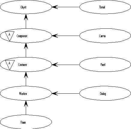
The design of the PetriTool application consists of 27 classes. Design diagrams describing the interaction of these classes is shown in Figures 3 through 8. In these diagrams, ellipses represent classes. A line with an arrow indicates that a class extends (inherits from) the class being pointed to. A line with a closed circle on the end indicates that a class 'has' another class, and a line with an open circle on the end indicates a class 'uses' another class. For example, in Figure 3, the Arc class extends the PetriComponent class as indicated by the line with the arrow. The DesignPanel class has anywhere from 0 to N objects of the Arc class, as indicated by the solid circle line with 0 and N on the ends. Both the PetriToolFrame and ControlPanel classes use the FileViewer class. Finally, the NewDesignDialog and the ReallyQuitDialog classes both extend the YesNoDialog class. Figure 8 uses an additional symbol to indicate an abstract class, which is the upside down triage surrounding an 'A'. This style of diagram is derived from (Booch, 1994).
Figure 3 shows all of the PetriTool classes and their organization. The classes defined for the PetriTool application can be broken up into three main categories: GUI, Simulation, and Analysis. The number of classes making up each of these is 19, 1, and 5 respectively. The PetriTool and OptionsFrame classes are used for all of these functions.
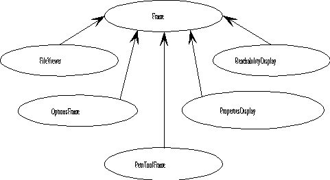
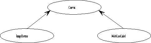
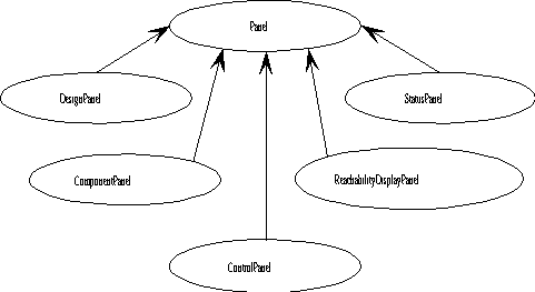
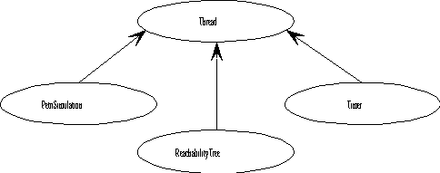
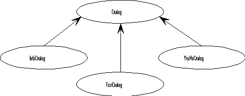
Figure 4 shows which PetriTool classes are extended from Java's Object class. These are PetriTool and PetriComponent. Figure 5 shows that five classes are extended from the Frame class and they are FileViewer, OptionsFrame, PetriToolFrame, PropertiesDisplay, and ReachabilityDisplay. The ImageButton and MultiLineLabel classes extend the Canvas class, as shown in Figure 6. Five classes are extended from the Panel class, as shown in Figure 7, and they are DesignPanel, ComponentPanel, ControlPanel, ReachabilityDisplayPanel, and StatusPanel. Figure 8 shows that three classes are extended from the Thread class and they are PetriSimulation, ReachabilityTree, and Timer. Figure 9 shows that the classes InfoDialog, TextDialog, and YesNoDialog extend the Dialog class. Finally, Figure 10 shows how the basic Java classes Object, Component, Container, Window, Frame, Thread, Canvas, Panel, and Dialog are related in the class hierarchy.

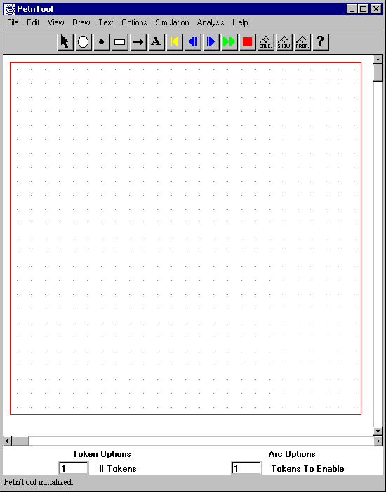
The Graphical User Interface for the PetriTool application consists of five major components. These components are the Menu Bar, Control Panel, Design Panel, Component Panel, and Status Panel. The Menu Bar consists of a set of drop down menus at the top of the window where the user can select various functions. The Control Panel, just below the Menu Bar, is a Panel of Image Buttons which can be depressed to select functions. All Control Panel buttons duplicate functionality that is available in the Menu Bar, but provides more convenient access to these functions. The Design Panel is the drawing area for the Petri net design, in the middle of the screen, just below the Control Panel. It is made up of a grid of spaces where Petri net components can be placed, and scrollbars on the right and bottom to move desired parts of the design into view. The Component Panel is just below the Design Panel. It provides an easy interface for selecting options for Petri net components that are drawn in the Design Panel. Finally, the Status Panel is a message board at the bottom of the window where the PetriTool application relays important information to the user regarding errors, hints for operation, and the basic status of the PetriTool methods. In Figure 11 below, all of these parts of the GUI can be seen.
The Menu Bar is made up of nine separate pull-down Menus. These
Menus are File, Edit, View, Draw, Text, Options, Simulation, Analysis,
and Help. Figure 12 below shows a close-up of the Menu Bar.

The first menu on the Menu Bar is the File menu. Figure 13 below
shows what the File menu looks like when it is opened.
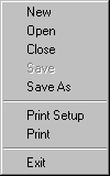
Under the File Menu, the New menu item clears the current design and leaves a blank Design Panel. Any current design on the screen will be lost unless previously saved, so a window will appear before clearing the design to confirm the New action. The user can select either Yes to continue with the New, or No to abort the New design action.
The Open menu item will read a previously saved PetriTool design into the Design Panel. The current Design Panel is first cleared of all components. Once a design file has been opened in this fashion, the Save menu item becomes enabled (Note that in Figure 13 above, Save is currently disabled.)
Once a design has been saved using the Save As menu item, or has been opened using the Open menu item, a file name and directory name are established and the Save menu item becomes enabled. Once enabled and it is chosen by the user, the design currently in the Design Panel is saved to that file name and directory.
The Save As menu item can be chosen at any time to save the current design. A File Dialog window will appear and allow the user to navigate through the directory tree and to select a file name to save the design as.
The Print and Print Setup menu items are not currently implemented. The current method for getting the PetriTool designs to the printer is to use third party screen capture utilities, which are available as freeware from the Internet. See Appendix A for a list of Internet sites and freeware titles that can perform these tasks.
Finally, the Exit menu item ends the current PetriTool application session. Since this will cause the current design to be lost if not yet saved, a ReallyQuitDialog window will appear and prompt the user to make sure the exit is actually desired. A response with the Yes button will end the PetriTool application, and a No button will abort the Exit command and return the user to the application.
The next menu on the Menu Bar is the Edit menu, shown in Figure 14.
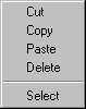
To begin any editing, the user must first select all components to be edited. This can be done by choosing the Select menu item. Once this is done, the user is given the Pointer in the Design Panel and may select components by clicking the left mouse button while over the object. Objects that are currently selected will appear with small green squares defining the area of the selected objects. For instance, places, tokens, transitions, and captions will have four green squares, one in each corner of the component. Arcs will appear with a green square at each of the two ends of the arc. In a similar fashion, selected components can be unselected by clicking anywhere within the area of the component.
Once the desired components are selected, the user may choose Cut, Copy, or Delete from the Edit menu. The Cut menu item will result in all currently selected components being removed from the design and placed in a temporary buffer. These components can be placed back into the design by choosing the Paste menu item described later. The Copy menu item will make a copy of all currently selected components in the Design Panel and place that copy in a temporary buffer, leaving the selected components in the design.
The Delete menu item will simply remove all selected components from the design, without copying them to the temporary buffer. In addition, when using Delete, some components are automatically selected for deletion. When deleting places, any tokens contained within the places are automatically deleted, as well as any arcs coming into or out of the place. When deleting transitions, incoming and outgoing arcs are also automatically deleted.
After components have been either Cut or Copied to the temporary buffer, the user may select the Paste menu item to put them back into the design. This is done by first selecting the Paste menu item, which will automatically select the Pointer button. The user will then click the mouse button at the location where it is desired to place the components. The grid square that is selected by the user will be the location of the upper left hand coordinates of all selected components. The PetriTool application will check the destination of all of the Pasted components to make sure there will be no overlapping of existing components in the Design Panel, and that components do not span beyond the border of the Design Panel. A message in the Status Panel will appear to inform the user if these conditions occur, and prompt for a different location to be chosen.
The next Menu Bar menu is the View menu, as seen in Figure 15.
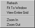
There are five menu items in the View menu: Refresh, Fit To Window, View Entire Grid, Zoom In, and Zoom Out. Refresh is used to redraw the entire PetriTool application window. This is useful when the windows of other applications hang and leave behind parts of their window and do not redraw the PetriTool application. A redraw is built in to the PetriTool application to handle the normal situations where windows will be drawn or moved across the PetriTool window, or when the PetriTool window itself is moved, resized, iconified, and deiconified.
The Fit To Window menu item will make the Petri net design as large as possible and still fit within the current window, and with the grid squares remaining square, as opposed to stretching to a rectangular shape. The Fit To Window does not account for Caption text when performing the resizing. This was desired in order to allow for comments to appear anywhere throughout the Design Panel, and still allow the Fit To Window to enlarge the important components of the design.
The View Entire Grid menu item is used to bring the entire design sheet into the current window, and making the design sheet as large as possible. This is a useful tool for being able to quickly zoom out of any view and to be able to see the entire design.
The Zoom In and Zoom Out menu items will enlarge or reduce, respectively, the size of the Petri net components by a factor of two, allowing the user to focus on specific areas of a larger design.
The next Menu Bar menu is the Draw menu seen in Figure 16.

The Draw menu contains all the menu items needed to add components to the Petri net design, including places, tokens, transitions, arcs, and caption text.
To add a place or transition to the design, the user will select either the Place or Transition menu item, then click the mouse button in the grid square where the component should be drawn. Note that the PetriTool application will not allow places or transitions to be drawn outside the border of the Design Panel, or within one grid square of other places or transitions. This is enforced so that the resulting design has a more organized and clean appearance.
To add a token to the design, the user can select the Token menu item, then click the mouse button in the Design Panel over the place component where the token is to be added. The number of tokens added to that place will be the number of tokens specified in the Component Panel (the panel between the Design Panel and the Status Panel as seen in Figure 11) under the Token Options heading. The PetriTool application will not allow tokens to be drawn outside the Design Panel border, in grid squares that do not contain Places, or in grid squares that already contain tokens. However, when using the Cut, Copy, and Paste functions, these rules are not enforced, allowing the user to edit a design without restriction.
To add an arc to the design, select the Arc menu item from the Draw menu, then click and hold the mouse button on either a place or transition component and drag it to another transition or place component. Whether or not the arc is an input or output arc of a transition is determined by which direction the mouse is dragged. The arrowhead of the arc is always drawn at the ending component, so that if you drag the mouse from a place to a transition, the arc will be an input arc of the transition. The number of tokens needed to enable the arc will be the current value of the "Tokens To Enable" field of the Component Panel under Arc Options. When the arc is complete, this value will be shown by a slash mark through the arc with a number next to it representing the number of tokens it will take to enable the arc. The PetriTool application will enforce the restriction that arcs must be drawn between a transition and a place, so it is not possible to have an arc drawn between two places or two transitions, or from a place or transition to an empty grid square.
In order to add comments to the design, the user can select Text from the Draw menu. When this is done, a Text Dialog box appears which provides the user with a TextField to enter their comments in, and an OK button to accept the text or a Cancel button to reject the text. A picture of the Text Dialog box can be seen in Figure 17.

After the user has entered some text and selected the OK button, the Pointer button on the Control Panel is automatically selected, and the user is prompted to select a location for the text. To pick a location, the user simply needs to click the mouse in the grid square where the bottom left hand corner of the text is to appear. The PetriTool application will prevent the user from selecting a location outside of the Design Panel border, or a location that would start within the border, but would span outside the border by the end of the text.
Using the Text menu from the Menu Bar, the user can select how the text captions described in the previous section are drawn. Figure 18 below shows what the Text menu looks like. The first menu item is Font Style, which is actually a list of CheckBox Menu Items, one for each Font Style that is available. The user selects the font by clicking on the desired Font Style, which automatically unselects all other Font Styles.

In a similar fashion, the user can select the size of the caption text using the Font Size menu item which lists all of the available sizes for the Font.
The next three menu items determine the emphasis of the Font. Their are four possible combinations for emphasis which are Regular, Bold, Italic, or Bold Italic. The user simply clicks the mouse next to the desired emphasis selections. Note that the Regular menu item is mutually exclusive with respect to both the Bold or Italic menu items.
The next Menu Bar menu is the Options menu, which currently holds one menu item, Preferences, as seen in Figure 19 below.

Selecting the Preferences menu item will cause the PetriTool application to bring up a window with a wide assortment of options available for the application, including Color, Grid, Analysis, Simulation, and Miscellaneous option groups. At any time, the user can select the OK button to accept the current options, the Default button to load the default settings for all the options, or the Cancel button to exit the Options window without making any changes. Figure 20 shows the color options available through the Options menu. The user has a separate list of colors to choose from for the foreground color, background color, grid color, border color, and caption color. The colors available for each of these items is: black, blue, cyan, dark gray, gray, light gray, green, magenta, orange, pink, red, white, and yellow. The default color settings are shown in Figure 20.
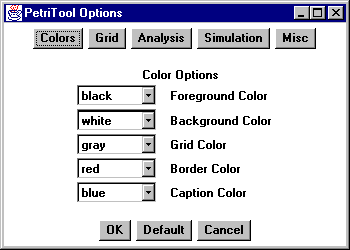
Figure 21 below shows the options that are available for the grid. The user can select whether or not to show the grid points in the Design Panel, and may also select the height and width (in grid squares) the Design Panel should be. The available sizes for each are: 10, 15, 20, 25, 30, 35, 40, 45, and 50. The default values are shown in Figure 21.
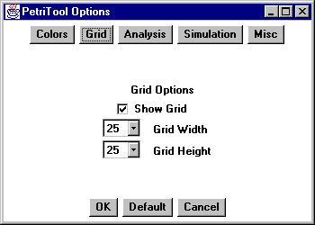
Figure 22 shows the analysis options the user may select. The user may opt to set a limit on the amount of time it takes to create the reachability tree, and may also select that time in minutes. The available time choices include 1, 5, 10, 30, 60, 240, and 480 minutes. The default settings are for the analysis time to be bound at 1 minute.
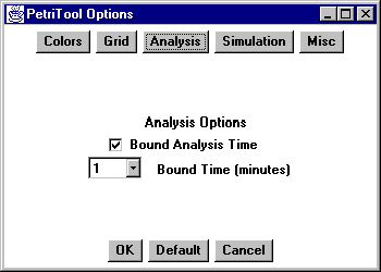
Figure 23 shows the simulation options available to the user. The simulation speed is the amount of time the simulator pauses at the marking phase, and at the phase where the activated transitions are highlighted. See the Simulation section for more detail. The simulation speed scale ranges from 1 to 10, with 10 being the fastest and 1 being the slowest. Table 5 below shows how the various speed setting relate to the amount of time the simulator pauses.
|
|
|
|
|
|
|
|
| |
The history size option is the number of simulation steps the PetriTool simulator will keep in memory so that the user can reverse step through past simulation cycles. The history size can be set to 10, 25, 50, 75, 100, 200, 250, 300, 400, and 500 simulation cycles. The default simulation options are shown in Figure 23.
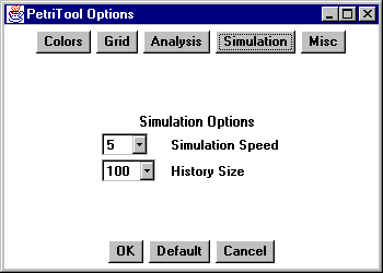
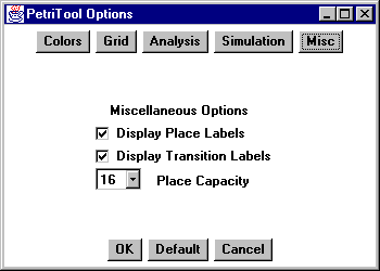
Figure 24 shows the set of miscellaneous options that are available to the user. The user can select whether or not the place and transition labels are displayed in the Design Panel. The user can also select the maximum number of tokens that may reside in a place at any given time, known as the Place Capacity. This value is used during the drawing of the design, limiting the number of tokens that the user initially adds to a place. This number is also used during simulation, where the number of tokens that are deposited in a place will not exceed the place capacity. Finally, this number is used during analysis to limit the infinite number of markings that could be created with a place that is unbounded. The possible settings for Place Capacity are 1, 2, 3, 4, 5, 6, 7, 8, 9, 10, 11, 12, 13, 14, 15, 16, and 32. See the Analysis section for more detail.
The Simulation menu of the Menu Bar is shown in Figure 25 below. There are five functions which can be selected from the Simulation menu including Reset, Forward Step, Reverse Step, Run, and Stop.
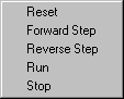
The Reset menu item resets all the tokens to their initial marking. Anytime a token or place is added to the design, a new initial marking is defined, and it is this marking that the Reset function will use. The Reset will also clear the history Vector used for Reverse Step operations.
The Forward Step menu item will sort the transitions of the design by a weighting factor of how many times the transition has been activated vs. the number of simulation cycles that have occurred. A second sorting of the transitions will occur that will position all selected transitions to the front of the list, giving them higher temporary priority while they are selected. The Forward Step procedure will then traverse the list of transitions and activate the transitions if they are enabled. Once it has been determined which transitions will be activated, the PetriTool simulator will color all activated transitions to indicate to the user which transitions are firing. The appropriate number of tokens will be deducted from all of the source places. The simulator will then pause for an amount of time as determined by the Simulation Speed. After a brief pause, the simulator will return all transitions to their original color and add the appropriate number of tokens to all destination places. The simulator will then record the set of transition activations in the history stack and return control of the PetriTool application to the user.
The Run command simply makes continuous calls to the Forward Step routine, followed by the appropriate pause as specified by the simulation speed setting, until the user selects the Stop menu item. The Reverse Step menu item will pop the last saved set of transition activations off the history stack and perform the Forward Step routine in reverse order. If there have been no calls to the Forward Step or Run routines since, the Reverse Step routine will inform the user that there are currently no entries in the history stack.
The Analysis menu contains four menu items: Calculate Reachability Tree, Show Reachability Tree, Net Properties, and Search Reachability Tree. Figure 26 below shows the Analysis menu.
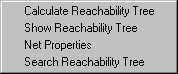
The first step in any analysis of a Petri net design is to construct the reachability tree, so the user must first select Calculate Reachability Tree before performing any of the other three analysis actions. The user will be prompted with a message in the Status Panel noting this procedure if any of the last three options are selected before constructing the reachability tree.
The algorithm used for constructing the reachability tree starts with an initial marking. From that point, a marking is created for all possible transition firings. These new markings are added to a Vector of markings to be solved. If a marking is reached that is already solved, an asterisk is placed next to that marking, and it is not placed in the pool of markings to be solved. The process repeats until the pool of markings to be solved is empty. At this point the tree is complete. After the tree is completed, a window will appear with the reachability tree and user can use scrollbars to view different portions of the tree.
Once a reachability tree has been constructed, the user can use the Show Reachability Tree menu item to bring up the window to view the tree, eliminating the need to reconstruct the tree.
The Net Properties menu item will analyze the reachability tree for the important Petri net properties including liveness, boundedness, conservativeness, and safeness. In addition, the Net Properties routine will indicate if there was an overflow condition in any of the places. An overflow occurs when the number of tokens in a place would have exceeded the maximum place capacity if the analysis were allowed to exceed that limit.
The safe and bound properties are closely related, with the safeness property being a more specific case of boundedness. A place is declared safe if, for all markings, the number of tokens contained within that place never exceeds one. The Petri net itself is declared safe if all of the places in the net are safe. A place is k-bounded if, for all possible markings, the number of tokens in that place cannot exceed k. In any case where a place is k-bounded and k = place capacity, the user must check the Overflow section of the properties list to make sure the place is truly k-bound. If there was an overflow for that place, it is not truly k-bound.
Another important property for Petri net analysis is conservativeness. The Petri net is declared strictly conservative if, for all markings, the total sum of all tokens always remains the same.
Finally, the reachability tree is analyzed for liveness. The Petri net is declared live if all of the leaves of the net are markings which exist somewhere previously in the net. Therefore the net is not live if there exists a marking within the reachability tree which has no enabled transitions.
The last menu of the Menu Bar is the help menu (Figure 27) which contains two menu items About and Select Item. When the user selects the About menu item, a window appears which indicates the current version and author information for the PetriTool application. When the user chooses the Select Item option, the Help button on the Control Panel is enabled and the user is prompted to select a button or menu item for which help is desired. After selecting any menu item or button, a help file for that option is opened and displayed in a window. When the user is done with the help file, they may select the Close button at the bottom of the window to dismiss the window.

The Control Panel for the PetriTool application brings the most commonly used functions forward so that they are more easily accessibly. Here, the user may perform all functions of the Draw and Simulation menus, as well as most of the Analysis menu functions and the Select Item of the Help menu. The Control Panel is shown in Figure 28.

From left to right, the Control Panel buttons are: Select, Draw Place, Draw Token, Draw Transition, Draw Arc, Draw Text, Simulation Reset, Simulation Reverse Step, Simulation Forward Step, Simulation Run, Simulation Stop, Calculate Reachability Tree, Show Reachability Tree, Net Properties, and Select Item for help.
The Design Panel of the PetriTool application is where most of the activity occurs. The Design Panel appears as a grid of squares in which Petri net components can be placed. The number of grid squares wide and high can be customized by the user through the Options menu item of the Menu Bar. Around the outside of the Design Panel there is a solid line border which defines the boundaries of the design area. There are also scrollbars on the right side and on the bottom of the design panel to view designs which may not fit entirely in the window of the PetriTool application.
The Component Panel is a panel at the bottom of the PetriTool window, just above the Status Panel. The purpose of the Component Panel is to allow the user quick an easy access to variables that may be set for each Token and Arc component that is drawn on the Design Panel. Figure 29 shows how the Component Panel appears in the PetriTool application.

For tokens, the user may select the number of tokens they wish to add to the design. In order to preserve the simplicity of the design, when tokens are added to a place, only a single graphical token is drawn, but this graphical token may represent a variable amount of actual tokens, which will be indicated by a text string underneath the token (i.e. "T = 2" for two tokens).
For arcs, the user is able to select the number of tokens that are required to enable the arc. The number selected will appear next to a slash mark on the arc about halfway down its length.
The Status Panel, as seen in Figure 30, is where the PetriTool application will send status messages to the user. The intent of the Status Panel is to display not only errors, but also inform the user of what is being done wrong, and in some cases suggest a course of action to correct the problem. This is an area of improvement over other tools available which seemed at times to lack this user friendly quality.

Table 6 shows all of the possible Status Panel messages that the
user can receive.
| ComponentPanel.java | Invalid value for 'Tokens To Enable', using 1 instead |
| # Tokens exceeds Maximum Place Capacity, using Maximum Place Capacity instead | |
| Invalid value for '# Tokens', using 1 instead | |
| ControlPanel.java | Error loading image 'imageName.gif' |
| Error opening help file | |
| Move the cursor to a Petri net component and press a mouse button | |
| Move the mouse to the desired position, click the mouse button to draw a Place | |
| Move the mouse to the desired Place, and click the mouse button to add a Token | |
| Move the mouse to the desired position, and click the mouse button to add a Transition | |
| Move the mouse to the desired position, and click and hold the mouse button to add an Arc | |
| Please type your caption text in the dialog box | |
| There is no simulation initialized, select Reset, ForwardStep, or Run | |
| There is no simulation or analysis currently running | |
| Calculating the reachability tree... | |
| No reachability tree currently constructed, try Calculate Reachability Tree first | |
| Please type the marking to search for in the dialog box | |
| Choose a component, menu or button to get help about it | |
| Error saving file, bad file name 'someFile.pnt' | |
| Print Setup option not yet implemented | |
| Print option not yet implemented | |
| There were no components selected to cut | |
| Screen Refreshed | |
| Zoom Out | |
| Cannot zoom out any further | |
| Zoom In | |
| Cannot zoom in any further | |
| DesignPanel.java | Saving to file 'fileName.pnt' |
| Error saving design | |
| Opening file 'fileName.pnt' | |
| Error loading design | |
| New design initialized | |
| Components overlap, select another destination | |
| Components span beyond border, select another destination | |
| Captions may not be drawn within 1 grid space of other elements | |
| Caption dimensions extend beyond border | |
| Captions must be drawn within the border | |
| Places may not be drawn within 1 grid space of other elements | |
| Places must be drawn within the border | |
| Tokens already occupy this Place | |
| Tokens must be drawn within Places | |
| Tokens must be drawn within the border | |
| Transitions may not be drawn within 1 grid space of other elements | |
| Transitions must be drawn within the border | |
| Arcs must start at either a Place or Transition | |
| Move to the desired end position and release the mouse button | |
| Arcs must be drawn within the border | |
| Arcs cannot be drawn between the same component | |
| Arcs must end within the border | |
| Arcs must end at either a Place or Transition | |
| Arcs cannot be drawn between like components | |
| An Arc is already placed there | |
| Validating design, please wait... | |
| The design contains a dangling Token at x = 'x Coordinate', y = 'y Coordinate' | |
| The design contains an unconnected Place at x = 'x Coordinate', y = 'y Coordinate' | |
| The design contains an unconnected Transition at x = 'x Coordinate', y = 'y Coordinate' | |
| The design contains an unconnected Arc at x = 'x Coordinate', y = 'y Coordinate' | |
| Design is valid | |
| NewDesignDialog.java | New design canceled |
| PetriSimulation.java | No Transitions are enabled, simulation cannot proceed |
| The history size is currently 0, cannot Reverse Step | |
| Design is not valid | |
| ReachabilityTree.java | Analysis Timer set for 'someNumber' minute(s). |
| Analysis was interrupted before completion, reachability tree may be incomplete | |
| Reachability tree could not be constructed in the amount of time specified in Bound Time | |
| ReallyQuitDialog.java | Quit canceled |
The design of the simulation module of the PetriTool application consists of a single object, PetriSimulation, which encapsulates all of the simulation functionality and extends the Thread class. A new PetriSimulation object is created, if one does not already exist, when the user selects either Reset, Forward Step, or Run. Anytime a new component is added to the design panel, the PetriSimulation object is destroyed, so that these new components can be initialized and incorporated into further simulation steps. The user must then start the simulation over by again selecting Reset, Forward Step, or Run.
The main routine of a Java Thread is the run() method. For the PetriSimulation object, the activity in the run() method is based on a modeString_ which indicates that the simulation is either in a Forward Step mode, Reverse Step mode, Run mode, or Stop mode. After a single step forward or reverse, the run() method sets the modeString_ to Stop which suspends the thread. The thread also goes into Stop mode and suspends when the user selects the simulation stop button.
The PetriSimulation object will activate transitions in the design based on the weight of each transition according to a fairness algorithm. Initially all weights are zero so all transitions have an equal chance of being activated. Each transition has an activation counter which is incremented for each simulation cycle that it is activated. Before each simulation cycle, the activation counter of each transition is divided by the number of simulation cycles that have passed since the simulation started, which becomes the weight for that transition, represented as a double. The Vector of transitions is then sorted, with the lowest weighted transition placed in the front of the Vector up to the highest weighted transition at the end of the Vector. At this point, priority transitions are sorted as described in the next section.
The user may give priorities to transitions which will supersede the weights assigned based on the fairness algorithm. In order to give a transition priority over a transition competing for the same tokens, simply use the pointer function to select the transition, in the same way that is done to select objects for the editing functions. Once the transition is selected, it will be surrounded by the bounding box consisting of the green squares at each corner of the component. During each step of the simulation, the transitions will first be sorted by their weights, and then all the selected transitions will be brought to the front of the sorted Vector. The result will be that at the beginning of the transition Vector will have the selected transitions sorted by weight, then the unselected transitions following those which will also be sorted by their weight. An example of a transition with priority is shown below in Figure 31.
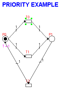
In this example, transitions T0 and T1 are competing for the token in place P0. Normally, the transitions will be activated in an alternating fashion. However, with T0 selected as depicted in Figure 31, T0 will always be activated by the token in place P0 and transition T1 will never be activated. It is important to note that the user may stop the simulation at any time and select or unselect transitions then resume simulating from the current marking without having to reset the simulation. Components other than transitions which are selected will have no affect on the simulation.
A reset is executed automatically the first time a Forward Step or Run is performed, or can be executed manually by the user by selecting the Reset button or menu item. The purpose of the reset is to set up all necessary variables and pointers for the simulation.
The first step of any reset is to make sure that the design is valid by making a call to the validDesign() routine of the Design Panel. This routine will check for any dangling places, tokens, transitions, and arcs. Dangling places and transitions are places and transitions that have no incoming or outgoing arcs. A dangling token is a token which does not reside in a place. Finally, a dangling arc is an arc which does not have either a place or transition at both ends.
If the design is valid, the reset continues by setting the current marking equal to the initial marking. All tokens are first removed, then added according to initial marking. Transitions are reset by setting the number of times they have been activated to 0, their current weight to 0, and set them to not be enabled.
Next, four Vectors are set up for each transition in the design. These Vectors are the sourcePlaceVector_, tokensNeededVector_, destinationPlaceVector_, and tokensDistributedVector_. The sourcePlaceVector_ contains a pointer to each of the places that are sources for the transition, with the tokensNeededVector_ containing the integer number of tokens needed from each place to enable the transition. The destinationPlaceVector_ contains a pointer to each place that is an output of the transition with tokensDistributedVector_ containing the integer number of tokens that are added to each of the places after the transition has fired. Although the creation of these Vectors adds slightly to the memory requirements of the application, it does eliminate the need to setup up each of these pointers at each simulation cycle and also simplifies the simulation algorithm.
The last function of the reset is to start a history Vector to contain a list of transition firings for later use by the Reverse Step function. After this has been done, the reset() method sets the modeString_ to "Stop" then starts the run() method which will suspend the Thread until the user selects a Step or Run button.
Forward step allows the user to activate one set of transitions and see the change in markings. Both the Forward Step and Run procedures use the goForward() method of the PetriSimulation object. The algorithm used for the goForward() method starts by calling the setActivationWeights() method to set the weights for each of the transitions. The sortTranstions() method is then called to order the transitions based on their weights.
Once the transitions have been ordered, the goForward() method will determine, for each transition, if it is enabled. This is done by calculating if, for each place in the sourcePlaceVector_, the number of tokens required from those places, as stored in the tokensNeededVector_, are present in the places. If this is true, the transition is set to enabled and the tokens are deducted from the source places. These tokens will be unavailable for transitions with higher weights which will be further down in the ordered Vector of transitions.
At this point, the set of activated transitions is stored in the first element of the simulation history Vector. If the history Vector has reached its maximum size, the last element (oldest element) of the history vector is removed. The design panel is repainted at this point with all activated transitions colored red and the simulation will sleep() for the amount of time indicated by the simulation speed variable.
The second phase of the simulation cycle begins after the sleep() has been completed. For each of the activated transitions, each place in the destinationPlaceVector_ is given the number of tokens specified in the tokensDistributedVector_ for that place. All transitions are set to be not enabled, and the simulation repaints the Design Panel. All transitions will return to their normal color and the new marking will be shown. The simulation cycle number is then incremented.
If there were no activated transitions, the simulator sets the modeString_ to Stop and the simulation will suspend itself at the end of the cycle. This is done because once a simulation cycle occurs where there have been no activated transitions, it is not possible for future cycles to produce activated simulations. The net is deadlocked.
Run Simulation is accomplished by making a call to the goForward() method then calling sleep() for the amount of time specified by the Simulation Speed variable to allow the user to see the new marking. This is then repeated continually until the user chooses the Stop button or the net becomes deadlocked.
The user may use the Stop Simulation anytime the simulation is in Run mode. Internally, this is accomplished by setting the modeString_ to Stop, which is handled in the run() method by suspending the PetriSimulation thread.
The Reverse Step method will first check to see that there is at least one element in the historyVector_. If there is at least one element, the first element in the Vector is removed. The historyVector_ element contains a list of transition firings. Each of these transitions is activated and tokens are removed from each of the places in the destinationPlaceVector_, with the number of tokens to be removed indicated by the tokensDistributedVector_. The design panel is then repainted to show the activated transitions shown in red. The simulation thread then calls sleep() for the amount of time indicated by the simulation speed variable. Tokens are then added to each of the places in the sourcePlaceVector_ for each activated transition, with the number of tokens added specified in the tokensNeededVector_. All transitions are set to be not enabled, the Design Panel is repainted again to show the new marking, and the simulation cycle count is decremented.
The ability to analyze Petri nets is generally considered to be the most important activity. Through the analysis of a Petri net, the designer can gain insight into the behavior and properties of the modeled system. There are two major types of analysis that may be performed on Petri nets. The first involves the creation of a reachability tree, and the other involves matrix equations. There are tradeoffs involved with selecting a particular analysis technique, but the reachability tree method was chosen for this project.
Use of matrices to analyze Petri nets has a number of disadvantages which make an automated solution difficult for a large class of Petri nets. The matrices do not reflect the actual structure of the Petri net, causing problems with canceling terms when transitions have both inputs and outputs from the same place. There is no sequencing information in the firing vector, so that a sequence of T1T2T3 is the same as T1T3T2 for example. Finally, solving the matrix equations provides a solution which is necessary for reachability, but not sufficient, and is known to produce spurious solutions (Peterson, 1981).
The reachability tree can effectively solve the safeness, boundedness, and conservation properties. The problems arise when using the reachability tree when there exist loops in the tree which cause a particular place to be occupied with an infinite number of tokens, which results in an infinitely sized tree. An example of such a Petri net is shown in Figure 32.
This tree has an initial marking of (1,0) and after transition T0 fires becomes (1,1), then after T0 fires again becomes (1,2), and so on up to (1,). The method proposed described in (Peterson, 1981) is to identify such markings and replace all markings from (1,1) to (1,) with one marking (1,). This would result in a tree with two markings, (1,0) and (1,). This at least allows the reachability tree to be created, however it results in a loss of information which excludes the possibility of analyzing the tree for the liveness property. It also makes it impossible to see what sort of transition firing sequences are possible.
In the PetriTool application, a slightly different method is used to get around the infinite marking problem. A maximum place capacity is specified by the user, so once the number of tokens in a place reaches that capacity, adding tokens does not increase the token count. If the capacity of a place would be exceeded in the complete net, then this is flagged as an overflow for that place. For the net in the above example, if the user specified a place capacity of 16, the reachability tree would consist of markings (1,0), (1,1), (1,2), up to (1,16). Place P1 would be flagged as having an overflow because there are actually additional markings possible in the complete net, i.e. (1,17) through (1,)..
The construction of the reachability tree is the first step in any analysis of the Petri net. A reachability tree is constructed by creating a ReachabilityTree object, which is a separate Java Thread. The constructor for the ReachabilityTree object will perform all necessary initializations and start the analysis. When finished, it will automatically display the reachability tree.
The first important step for creating the reachability tree is to setup some information in each of the transitions. This initialization is performed in a method called initializeTransitionMarkings(). This routine sets up two Vectors in each transition, each Vector with as many entries as there are places in the Petri net. The first Vector is called the changeMarking_. The entries of this Vector are integers corresponding to the change in the number of tokens in each place when the transition fires. For example, a change marking of (1, -1, 0) for some transition T0 would correspond to a three place Petri net that, when T0 fires, adds a token to place P0, removes a token from place P1, and has no effect on place P2.
The next Vector which is setup for each transition in the initializeTransitionMarkings() method is a needMarking_. This Vector has as many entries as there are places in the Petri net, and corresponds to the number of tokens required from each place in order for the transition to fire. For example, a needMarking_ of (0, 1, 0) for some transition T0 would indicate that the transition needs one token from place P1 in order to fire, but none from places P0 and P2.
The algorithm for constructing the reachability tree starts with one node, or marking, which is referred to as the initial marking. This marking is added to a Vector, toBeSolvedVector_, which holds all frontier nodes. Frontier nodes are nodes which have not yet been analyzed, and are created when transitions are fired from other frontier nodes. While the size of the toBeSolvedVector_ is greater than zero, the algorithm will remove an element from the Vector and call analyzeNode() with that marking as a parameter, which will generate more frontier nodes that are added to the toBeSolvedVector_. There are two other types of nodes which help to diminish the size of the toBeSolvedVector_. These are duplicate nodes and terminal nodes. Duplicate nodes are nodes which have already been analyzed and are already in the tree. These nodes need not be analyzed again because all successors to this marking will have already been produced from the first occurrence of the node in the tree. Terminal nodes are nodes or markings in which there are no enabled transitions, so no new markings can be created from them.
The analyzeNode() algorithm first checks to make sure the node it is analyzing is not already present in the tree. If it is not a duplicate, a booleanVector_ is created by a call to getTransitionFirings(). The booleanVector_ consists of a boolean value for each transition in the Petri net to indicate if it is enabled by the current marking. For each true element in the booleanVector_, a new marking is generated by using the transitions changeMarking_. This new marking is added to the toBeSolvedVector_. At this time, the algorithm also takes note of any overflows that occur.
If the user has selected to bound the analysis time, a Timer object will be created when the construction of the reachability tree begins. The Timer object is a Thread which will sleep() for the amount of time specified as the bound time. When the Thread wakes up, it will call the timerInterrupt() method of the ReachabilityTree object. The ReachabilityTree Thread will then terminate, if it is still running, and inform the user that the tree could not be completed in the amount of time allotted.
The safeness property is an important property to consider for a hardware design. If a place is safe, then the number of tokens in that place is guaranteed to be either 0 or 1. For a hardware design, for example, this might mean that the design can be implemented using a one bit register or flip-flop. However, note that the token may represent a larger entity in other designs.
The algorithm for calculating the safety of places starts by traversing the reachability tree and creating a maxTokenVector_. This Vector has an entry for each place in the Petri net which contains the maximum number of tokens that appeared in that place throughout the entire reachability tree. After this Vector is created, each place which has a maximum token count of 1 or less is declared safe. If all of the places in the net are declared safe, then the net as a whole is also declared safe.
The boundedness property is a more general case of the safeness property. It relaxes the requirement that the number of tokens in a place cannot exceed 1 to the more broad requirement that the number of tokens in a place cannot exceed some integer k. For a hardware design this implies that the place can be modeled by some known sized buffer or counter, with the guarantee that the buffer will not be overflowed.
The algorithm used to calculate the boundedness of each place starts out the same as the safety algorithm, by calculating the maxTokenVector_. This Vector is actually only calculated once, then used by each algorithm. The bound value for each place will be the maximum token count for that place. The bound value for the Petri net as a whole will be the highest entry in the maxTokenVector_.
The Petri net property of conservation is an important property for nets that model resources, such as a I/O devices. For these systems, where the tokens of the Petri net represent a system resource, it is important to be able to show that the number of resources, or tokens, remains constant.
The algorithm for determining whether or not the Petri net is strictly conservative starts by finding the sum of all tokens in the initial marking. Then, the reachability tree is traversed and the sum of all tokens is calculated for each marking in the tree. If all the markings in the reachability tree have the same sum of tokens, then the Petri net is declared to be strictly conservative.
The liveness property of a Petri net is also an important property to consider for nets which model communication protocols, resource allocation, or safety critical systems. It is important to be able to show that these systems will be able to run continuously without reaching a deadlock state.
The algorithm used to calculate whether or not the Petri net is live also involves traversing the markings of the reachability tree. If any marking exists in the tree such that no transitions are enabled from that marking, then that marking represents a deadlocked state, and the Petri net is declared to be not live. Otherwise it is declared live.
The term overflow is not a term that is generally used in reference with Petri nets, but was adopted in the PetriTool application in order to address the infinite marking problem. As was stated earlier, the PetriTool application solution to the infinite marking problem is to put a bounds on the maximum token capacity of a place. When the number of tokens in a place can exceed this maximum capacity, the place is flagged as having an overflow, but no markings are generated that have token counts over this capacity.
It is important that the user take note of places that are tagged as having an overflow, because this can affect the meaning of the other properties. The first property that overflows can have an affect on is the safeness property. For example, if the user selects a maximum place capacity of 1, all places will be tagged as safe because it is not possible for places to contain more than one token at a time. However, if a place is tagged as having an overflow, the place is not actually safe, and the Petri net as a whole is no longer safe as well.
The boundedness property must also be reviewed when there are places which had an overflow. Any place that is tagged as k-bounded, where k is also equal to the maximum place capacity must be observed. If any of these places had overflows, then the place is not actually k-bounded since the number of tokens contained in those places will exceed k in an actual design. It is up to the designer to determine the whether or not an overflow is significant for a particular place.
When PetriTool application files are saved to disk, all of the information needed to reproduce the design is saved, along with all of the user specified options regarding colors, grid, simulation, analysis, and the other miscellaneous options. Appendix B shows the design file for the Petri net design of Figure 1. Note that lines starting with a "#" are comment lines, and any number of comments may appear between sections, i.e. between the Place section and the Transition section. The file ends with a comment line "#END OF DESIGN FILE".
The design tradeoffs for this project can be broken down into four major areas. These are design strategy tradeoffs, GUI tradeoffs, simulation tradeoffs, and analysis tradeoffs.
The first tradeoff made was the choice of Java as the implementation language. Since Java is such a new language, bugs in the language were all but guaranteed. However, Java was still chosen for its cross-platform compatibility and automated garbage collection. Next, Café was chosen as a development tool for the project despite the fact that it too was a brand new tool with the existence of bugs being very likely. However, the tool provided a fast compiler and excellent project management facilities. Lastly, it was decided that the PetriTool program should be an application instead of an applet. This decision made the use of graphics a little more difficult, but had the advantage of eliminating the need for an applet viewer or browser to run the program, thus eliminating an additional source of bugs. Finally, the choice was made to use layout managers to construct the PetriTool application so that the program would be more platform independent. Although visual development tools were available, they placed components at fixed coordinates, changing the appearance of the program on different platforms.
The next set of design tradeoffs are concerned with the graphical user interface. The choice of implementing a grid based design panel instead of an unconstrained design panel was made. This limited components to specific squares on the design panel, instead of allowing them to be placed at precise coordinates. However, this design choice allowed for components to be uniquely and easily identified, and allowed for easier calculations within the program.
Next, it was decided that a single token object should be made to represent multiple tokens. Although this created a discontinuity with the natural identification of objects in the solution space, it provided numerous implementation benefits. Primarily, this decision saved memory space, having only one token object representing numerous Petri net tokens. It also provided for visual simplicity, graphically displaying only one token in a place, then having a text string to indicate how many actual tokens were occupying the place.
Arcs were designed to be objects with only two coordinates: a starting coordinate and an ending coordinate. This provided for an easy implementation, at the cost of limiting the design and making some designs more difficult to represent. After seeing how this limited the design ability of the PetriTool application, it was decided that this should be a high priority item for the next revision of the tool. Arcs were also implemented such that only one arc could connect the same two components in the same direction. In the case where multiple arcs are desired, the user must select the number of tokens it takes for a single arc to be enabled, thus saving memory by having only one arc object represent numerous arcs.
Transitions were implemented such that they were represented on the screen as rectangular shapes instead of the more popular line representation. This made it easier to draw arcs to the transition, and made it easier to show transition firings during simulation cycles.
Design decisions affecting zoom operations were also made. First, the Fit To Window command was designed so that captions were not accounted for when resizing the design in this manner. This allowed for comments, such as the author's name, date, etc. to be placed in the corner of the design, but still allow the user to focus on important Petri net components with this command. Also, it was decided to provide only Zoom In and Zoom Out commands for zooming, eliminating the 75% Zoom, 125% Zoom, etc. This was done because scaling fonts smaller and larger by a fractional factor caused the font size to grow larger and larger due to rounding errors.
There were also some design decisions made with respect to editing functions. First, the Delete function will auto select attached arcs and tokens for deletion when transitions and places are selected for deletion. This was done simply to speed the design process for the user. Also, strict Petri net properties are not enforced during editing operations. For instance, a place and an arc may be cut and pasted, leaving the arc unconnected at one end. Instead, the design is validated before a simulation or analysis is performed. This allows the user more flexibility while designing the Petri net, but still enforces Petri net rules when necessary.
Finally, some design decisions were made concerning the panels of the user interface. The ControlPanel was added, even though it only duplicates functionality within the menus, to provide a quicker interface to the most common functions. The StatusPanel was added so that messages may be continually displayed to the user without having to display additional Dialog windows. Finally, the ComponentPanel was added so that the properties of components could be easily specified in the main window.
The design of the simulator involved fewer design decisions that the GUI, with most decisions made simply to enhance user functionality. One of the important decisions, however, involved the use of multiple Thread objects to simulate the different Petri net components. It was decided to implement the simulator using a single thread at this time. This was done because the tool is designed to run on only one machine, and additional threads would only serve to complicate the algorithm and slow down the simulator. Also, there are currently problems with threads not terminating after they are done on the Windows 95 platform.
The first design tradeoff for the analysis module involved the use of the reachability tree instead of matrices. This was done because, at present, there was more information on analysis techniques based on the reachability tree, with automated analysis algorithms easier to design. The reachability tree also offered the ability to determine more properties for the Petri net design. The drawback to using the reachability tree method is the fact that the PetriTool application is hindered by the state-space explosion effect, so that very large designs cause memory limitations to be met before a solution can be found.
The Place Capacity variable was added so that infinite loops in a Petri net design could be easily identified and analysis time could be bounded, and still allow for the calculation of Petri net properties such as boundedness. This is not possible when using a method such as using a special symbol () to identify such markings, as is described in (Peterson, 1981).
Next, the reachability tree was represented in a vertical form rather than a true tree format in order to eliminate the complexity involved in calculating spacing and window sizing. The tree was also displayed on a Canvas object using the Graphics.drawString() method so that individual markings could be colored differently when the user searches the tree for a particular marking. This method uses more memory and is slower than simply showing a string in a TextArea, but it was necessary in order to provide the coloring.
A Show Reachabilty Tree function was implemented so that the application does not have to recalculate the tree every time the user wishes to view it. And lastly, a bound analysis time option was provided to the user in order to allow for the user to cleanly stop an analysis after a specified amount of time, to account for very large designs which might take several minutes to calculate.
The current version of the PetriTool application has met all expectations that had been hoped for, with only a few problems encountered. This section will address the final product in terms of the functionality of the PetriTool application, the effectiveness of the Java language for programming applications, the design tools used in the development of the PetriTool application, and the design process that was undertaken.
The PetriTool application allows for the design of the essential Petri net components that are common to all Petri nets. The tool may be used to design ordinary nets and non-ordinary Petri nets. Modifications and extensions to Petri nets that are not currently supported include timed nets, stochastic nets, predicate/transition nets, colored nets, and other forms of Petri nets which extend the basic Petri net model.
Ordinary Petri nets are nets which only contain arcs with a weight of one. The PetriTool application allows arc weights of one or more, so both ordinary and non-ordinary nets are supported. Subclasses of ordinary Petri nets include state machine, marked graph, free-choice net, extended free-choice net, and asymmetric choice nets. These types of nets are discussed in detail in (Murata, 1989).
There do exist limits on the size and complexity of the Petri nets that can be modeled using the PetriTool application. These limitations are difficult to quantify, but a characterization of certain types of designs which might cause difficulties will be made. Obviously, the amount of memory available to the PetriTool application will also be a factor limiting design complexity.
Since the method used by the PetriTool application to analyze the Petri net is the reachability tree method, the analysis should be able to be applied to all types of Petri nets. The disadvantage to this method, however, is that it involves the enumeration of all possible markings in the tree. For more complex designs, the number of possible markings grows exponentially as more tokens, arcs, transitions, and places are added to the design. This type of behavior in formal analysis has been described as the state-space explosion effect.
After some careful testing of various designs, the following observations were made about the effectiveness of the PetriTool application. Three designs from (Peterson, 1981) and one design from (Murata, 1989) were tested using the PetriTool application, with the results shown below in Table 7.
| Fig. 3.31 (Peterson, 1981)
Producer/Consumer, Buffer Size = 16 | ||
| Fig. 3.32 (Peterson, 1981) Dining Philosophers | ||
| Fig. 3.33 (Peterson, 1981) - Readers/Writers, readers bound to 32, 32 readers, 32 writers | ||
| Fig. 9 (Murata, 1989)
Communication Protocol |
These performance tests were performed on an IBM Aptiva running at 133 MHz with 48 Mbytes of RAM and 512 Kbytes of cache. Performance on these particular problems is quite good. In general, designs which were created with a particular purpose in mind perform well. However, some other generic designs were also tested. There was no intended purpose to the designs but to have a certain number of components interconnected. For a design with 1 Token, 10 places, 10 transitions, and 20 arcs which were connected in a ring of alternating places and transitions, the reachability tree with 10 nodes was created in 0.5 seconds. Adding an extra token to the design resulted in a reachability tree with 55 nodes, and was created in 1 second. Adding two more tokens (for a total of 4) resulted in a reachability tree of 715 nodes; this was created in 55 seconds. The trend here shows how the state-space explosion effect will reduce performance of the design. It can be concluded that as the number of nodes in the reachability tree approaches the memory limitations of the hardware, the PetriTool application will not be able to continue.
Another observation on types of designs that will take more analysis time are those designs which contain transitions which generate more tokens than they absorb. These types of designs generally tend to have far more reachable markings. The Place Capacity variable keeps this type of design in check for smaller designs, but larger designs may still have reachability trees with thousands of nodes.
The Java programming language is still in its infancy. At the present time, there are at least 35 known bugs actually listed by its creators, with conceivably scores more which are not listed, or which have not yet been found. The following URL lists these bugs: (http://www.javasoft.com/java.sun.com/products/JDK/1.0.2/KnownBugs.html). There are also scores of features in the accompanying libraries which are needed, but not yet implemented. Most of these bugs and missing features can be dealt with for the time being, but a few do cause problems even with the PetriTool application.
The first component that needs improvement is in the area of Threads. Currently, there are bugs on the Windows95 platform which cause programs with multiple Threads to not terminate. On the HP Unix platform, the implementation of Threads does not follow the typical model for a multithreaded machine. The Threads on this platform can only be run one at a time. The Java Virtual Machine does not swap threads in and out unless the programmer is careful enough with the design to place calls to the sleep() method at the appropriate locations.
The other major area for improvement in the Java language is in the AWT support library. The ability to be able to convert a graphics Component, including the Canvas and Panel classes, into a .GIF or .JPG file would be extremely useful. Any type of application program that is going to support graphics needs a way to export these graphics, not just be able to display them on the screen. Also, there should be some type of support in the AWT for interfacing with I/O devices, such as a printer. These interfaces need to be specified as part of a Java library so that applications can still be designed to be portable. For instance, the FileDialog class provides a platform independent interface to a system's file structure. A similar interface would be desirable for I/O devices such as printers. Finally, the Scrollbar class, as implemented on the Windows95 platform, still contain bugs. The setPageIncrement() and setLineIncrement() methods seem to have no effect. Also, setting the size of the scrollbar to scroll through the appropriate sized area does not seem to work, resulting in a poor design.
Commenting on the effectiveness of the garbage collection ability of the Java Virtual Machine is difficult without a more extensive analysis. It would be necessary to have tools to see what objects have been freed vs. objects that should have been freed, or other methods of detecting memory leaks. The automatic garbage collection would seem to make real-time programs difficult to design, due to the lack of time constraint on when, how often, and how long the garbage collector would run for, although it is possible to force the garbage collector to run with a call to System.gc().
The portability of the Java code does seem to be very good. Different file systems are handled very well through the FileDialog class, and the AWT does a good job of keeping graphics components consistent across platforms. The use of Layout Managers is extremely important in achieving this consistency.
At this time, the maturity of the Java language seems to be able to handle some complex applications, however the existence of bugs and some missing features make it difficult at this time to recommend the language for use in situations where a program must be extremely robust.
The design of the PetriTool application was accomplished using the Café Integrated Development and Debugging Environment (IDDE) by Symantec Corporation and the Java Development Kit (JDK) by Sun Microsystems. The PetriTool application was designed, developed, and tested on a Windows95 platform. The program was also run on an HP Unix platform to verify cross-platform functionality. There do exist slight differences in appearance between the two platforms as a result of differences in the interpreters written for each platform, but all other functionality is the same.
When the PetriTool project began, the JDK 1.0 release had just been made, and the Symantec Café 1.0 release followed shortly thereafter. The newness of both of these products meant that bugs were likely to be present. The problem was further compounded by a lack of good documentation. Presently, the JDK is up to release 1.0.2 and Symantec's Café is currently on version 1.5.
The Symantec Café debugger was not used in the development of this application. This is mainly due to a lack of good documentation, and an initial requirement of having a TCP/IP connection active to use the debugger. Instead, the traditional method of print statements was used for debugging. The TCP/IP requirement has since been removed as of the 1.2 release, and there are now at least two third party books which document the Café development environment.
Another problem that was encountered initially with the Café program was with respect to the Windows95 screen resolution setting. With the highest resolution setting, the Café program would generate an error causing the program to crash. The error did not identify the source of the problem, and it cost a few days time to figure out the problem.
One important improvement that is needed for visual development tools in the Java arena is for these tools to be able to translate a visually created interface into layout manager format, instead of fixed positioning of components. It is for this reason that visual tools were not used to develop the PetriTool application.
The Café compiler, however, was an essential tool in the development of the PetriTool application. The Café compiler provided a substantial performance increase in terms of compile time over the standard JDK compiler, and has had benchmark results of ten times the speed of other Java tools (http://cafe.symantec.com/jit/analysis.html #benchcomp) . This performance increase meant considerably reduced debugging time. Café also had a good editor with syntax highlighting, search and replace, and support for emacs and other popular editor keystrokes which was a helpful feature, but no support for vi keystrokes. Overall, I believe the Café product considerably reduced design cycle time.
Another tool which helped to produce a well documented program is the javadoc program that comes with the JDK. This program extracted specially formatted program comments and generated HTML documentation for all of the Java source code written for the PetriTool application. This was a key utility for producing well documented code that will greatly reduce the time required for maintenance and upgrades.
Finally, the resources available over the Internet were an important tool due to the newness of the Java language and development tools. The comp.lang.java news group was read daily to get information on known bugs and examples of how to use some of the Java classes in the JDK libraries.
The final PetriTool application consists of 27 classes. Four of these classes were borrowed classes from other sources, and two are derived from the borrowed classes. The borrowed classes include FileViewer, InfoDialog, MultiLineLabel, and YesNoDialog which were borrowed from (Flanagan, 1996). Two classes are derived from YesNoDialog and they are NewDesignDialog and ReallyQuitDialog.
The design process began by identifying some of the more obvious objects. These objects include Arc, Caption, Place, Token, and Transition. All five of these classes are derived from a more general PetriComponent class which was developed to contain all of the common code for the five components.
Other objects were identified by breaking up the functionality and user interface of the program into logical parts. The main executable class is PetriTool, which creates PetriToolFrame to contain all of the elements of the GUI. The PetriToolFrame contains four panels, ComponentPanel, ControlPanel, DesignPanel, and the StatusPanel, each of which has its own well defined set of functionality. The ComponentPanel allows the user to specify parameters for the Petri net components being placed in the design. The ControlPanel provides a tool bar of ImageButtons and controls the functionality of the buttons. The DesignPanel provides a space for the user to design the Petri net, and includes methods to operate on the components of the design. Finally, the StatusPanel provides feedback to the user with error, hints, and explanations of the PetriTool's current state.
An OptionsFrame class was designed to provide a window with a wide assortment of user selectable options. Four other classes were developed to handle the analysis functions, ReachabilityTree, ReachabilityDisplayPanel, PropertiesDisplay, and Timer. And the PetriSimulation class was designed to handle simulation functions.
All of the classes composing the PetriTool application are fully documented with the standards defined by the javadoc utility, so that an HTML interface to all of the code could be automatically generated. This documentation, along with a clearly defined object oriented design results in a very maintainable application.
The PetriTool application is aimed at bringing together a collection of tools and features to the area of Petri net design, analysis, and simulation. The following two sections will discuss how well the goals of the PetriTool application have been met, as well as point out some future directions for updating the application.
There were numerous goals set forth for the PetriTool application. These goals included:
The goal of an effective user friendly interface is met through a collection of features. The tool provides easy access to the most frequently used tools by providing a toolbar consisting of ImageButtons which can be depressed to enable functions. The tool also provides a collection of editing features including Cut, Copy, Paste, and Delete to make the design process easier. The view of the design can be altered to zoom-in and zoom-out on portions of the design, with easy to use one touch zoom features such as Fit To Window and View Entire Grid. The screen can also be refreshed manually by the user. File operations are provided to allow the user to save and load designs from disk. Finally, the user is provided with a pop-up window full of options to customize the tool. These options include colors, grid options, analysis options, simulation options, and other miscellaneous options. The tool provides feedback to the user through the use of a StatusPanel which displays messages indicating errors, hints for correcting errors, and information on what the tool is currently doing. Help is provided through an interface where the user can select any feature on the tool with the click of a mouse, bringing up a window of help information about the feature. Overall, the PetriTool provides a very effective user interface, but there are improvements on the interface detailed in the Future Work section.
The tool provides analysis functionality based on the reachability tree technique. The tool provides the ability to construct and display a reachability tree, along with the ability to search the tree for a particular marking. After a reachability tree has been created, the user can extract the net properties including safe, bounded, live, and conservative. The user may also choose to bound the amount of time the tool should take to calculate the reachability tree, and also specify what that time limit should be.
The PetriTool application also provides a collection of simulation options which rivals current tools. The Petri net design may be run continuously forward, or stepped one set of transition firings at a time. The design may also be reverse stepped, an improvement over most current tools. The number of cycles that may be reverse stepped can be defined by the user. The user may also select the speed of simulation, which determines how long the simulator will pause before making the next set of transition firings. A reset feature allows the user to quickly return the design to its initial marking.
Maintenance can often be the most difficult task for a software engineer. The design of the PetriTool application aimed at easing the difficulty of the maintenance effort by adhering to good object oriented design practices, and by providing extensive comments. All comments throughout the PetriTool application's code adhere to the standards of the javadoc utility available as part of the JDK. This allowed the automatic generation of an HTML document which completely describes all PetriTool classes, variables, and methods.
One of the drawbacks to the current Petri net tools is that they are usually only available on one hardware platform, and when they are available on many platforms, it is through the laborious chore of porting the software, sometimes involving extensive rewriting. Because the PetriTool application is written in the Java programming language, it can be run, without modification, on any hardware platform that has the Java Virtual Machine ported to it. This is an excellent advantage for the PetriTool application, allowing it to reach the greatest number of end users. Also, any maintenance effort requires modifying only one set of source code to affect all platforms.
Finally, the last goal of this project was to prove that the Java language could be used to implement applications. This project has shown that the usefulness of the Java language can surpass simple applet enhancements to HTML pages, and provide a means of cross platform application development and maintenance that exceeds the ability of most other programming languages today. Nevertheless, the language is still very new, and will need to undergo further development to achieve acceptance in this area.
Although the current PetriTool application has met, and in some cases surpassed the initial requirements of the tool, there are areas where improvements and additions to the tool would enhance the GUI, analysis, and simulation functionality.
There are numerous additions and improvements that can be made to the graphical user interface. First, when drawing arcs the current PetriTool design panel will flicker as it repaints the panel as the arc is stretched from source to destination. It would be desirable to eliminate this flickering.
The next improvement would be to add printer capability to the tool as originally intended. If no support is offered through the JDK, then it would be useful to at least make print capabilities available on at least one platform through the use of hardware dependent system calls. Currently, the method used for printing a PetriTool design is to run a screen capture utility while the PetriTool application is running, select the area of the design to capture, then print the captured area using the screen capture utility.
The support for multi-point arcs and smooth curved arcs would also be an effective addition to simplify Petri net designs. Editing features that could be added include the ability to drag components on the screen, and to edit existing caption text. Keyboard shortcuts for menu items would also improve the GUI. Also, it would help to simplify designs if the place, transition, and arc labels could be moved by the user.
As far as simulation functionality goes, there are also a few improvements to be made in future revisions. First, it would be beneficial for the user to be able to disable certain transitions from firing during specific cycles of simulation. In addition, support for other types of transitions would extend the usefulness of the PetriTool application. Such transitions might include timed transitions, transitions firing based upon probabilities, and sink and source transitions.
Analysis improvements would include the ability to apply reduction rules on a specified net and the ability to perform timing analysis when timed transitions are added. Certain statistical calculations could also be added to make the PetriTool useful to Petri net designers interested in these characteristics.
Agerwala, Tilak. "Putting Petri Nets to Work." Computer
12.12 (Dec. 1979): 85-94.
Booch, Grady. Object-Oriented Analysis and Design. Second
Edition. Redwood City, California: The Benjamin/Cummings Publishing
Company, Inc., 1994.
Cornell, Gary, and Cay Horstman. Core Java. Mountain View,
California: Prentice Hall, Inc., 1996.
Flanagan, David. Java in a Nutshell. Sebastopol, California:
O'Reilly and Associates, Inc., 1996.
Murata, Tadao. "Petri Nets: Properties, Analysis and Applications."
Proceedings of the IEEE 77.4 (April, 1989): 541-580.
Peterson, J.L. Petri Net Theory and the Modeling of Systems.
Englewood Cliffs, New Jersey: Prentice Hall, Inc., 1981.
There are many freeware and shareware screen capture utilities available on the World Wide Web. Listed here are a few URLs and programs that exist. Also included are ways to find these and other screen capture utilities. Since the WWW is constantly changing, these may be even more useful since the utilities listed here may no longer exist and new ones may arise.
Try using these search engines with search phrases such as "Screen Capture" or "Windows 95 Screen Capture" for example.
The following pages are excellent resources for Windows 95 utilities.
The following page is actually where I was able to find three different screen capture utilities.
This appendix shows an example of the file format used to save PetriTool application design files. This file shows what the design of Figure 1 looks like.
# PetriTool v. 1.0
# Author: Rick Brink
#
# COLOR: background, foreground, grid, border, caption
white,black,gray,red,blue
# FONT: style, size, bold, italic
TimesRoman,10,true,false
# GRID: step, show, height, width
20,true,25,25
# SIMULATION: speed, historySize
5,100
# ANALYSIS: boundAnalysisTime, boundTime
true,1
# MISCELLANEOUS: placeLabels, transitionLabels, placeCapacity
true,true,16
#
# PLACES: x, y, label
Place: 7,6,0
Place: 7,12,1
Place: 3,15,2
Place: 12,10,3
Place: 12,14,4
Place: 17,6,5
Place: 17,12,6
Place: 22,15,7
#
# TRANSITIONS: x, y, label
Transition: 7,9,0
Transition: 7,15,1
Transition: 3,6,2
Transition: 17,9,3
Transition: 17,15,4
Transition: 22,6,5
#
# TOKENS: x, y, tokensRepresented
Token: 7,6,1
Token: 17,6,1
Token: 12,14,16
#
# ARCS: x1, y1, x2, y2, x1Draw, y1Draw, x2Draw, y2Draw, region,
tokensToEnable, slope
Arc: 7,6,7,9,0.5,1,0.5,0.25,2,1,1.#INF
Arc: 7,9,7,12,0.5,0.75,0.5,0,2,1,1.#INF
Arc: 7,12,7,15,0.5,1,0.5,0.25,2,1,1.#INF
Arc: 12,14,7,15,0,0.5,1,0.5,1,1,-0.2
Arc: 7,15,12,10,0.5,0.25,0.5,1,4,1,-1
Arc: 17,6,17,9,0.5,1,0.5,0.25,2,1,1.#INF
Arc: 12,10,17,9,1,0.5,0,0.5,3,1,-0.2
Arc: 17,9,12,14,0.5,0.75,0.5,0,2,1,-1
Arc: 17,9,17,12,0.5,0.75,0.5,0,2,1,1.#INF
Arc: 17,12,17,15,0.5,1,0.5,0.25,2,1,1.#INF
Arc: 7,15,3,15,0,0.5,1,0.5,1,1,0
Arc: 3,15,3,6,0.5,0,0.5,0.75,4,1,-1.#INF
Arc: 3,6,7,6,1,0.5,0,0.5,3,1,0
Arc: 17,15,22,15,1,0.5,0,0.5,3,1,0
Arc: 22,15,22,6,0.5,0,0.5,0.75,4,1,-1.#INF
Arc: 22,6,17,6,0,0.5,1,0.5,1,1,0
#
# CAPTIONS: x, y, actualSize, fontName, fontStyle, fontSize, ~^~captionText
Caption: 4,2,20,TimesRoman,1,20,~^~PRODUCER-CONSUMER EXAMPLE
Caption: 4,4,14,TimesRoman,1,14,~^~Producer
Caption: 18,4,14,TimesRoman,1,14,~^~Consumer
Caption: 10,17,14,TimesRoman,1,14,~^~Buffer Capacity = 16
Caption: 4,10,10,TimesRoman,1,10,~^~Produce
Caption: 19,10,10,TimesRoman,1,10,~^~Consume
# END OF DESIGN FILE